Improving predictions: My New Model

I’ve built a new model for predicting Premier League results. My aim was to minimise the mean absolute error (MAE) when predicting the result in an individual game. For example, if I predict a that Chelsea will beat Liverpool by 2 goals, but the result is a Liverpool win by 1 goal, the absolute error is 3 goals. Taking an average of all these errors over the same sample of games allows me to compare the accuracy of various models.

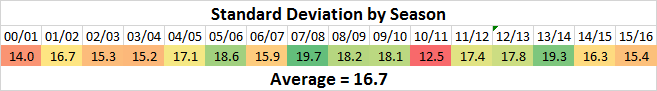
As a sample, I’m using Premier League results between 2001/02 and 2016/17. First, let’s establish a benchmark. If we guess that every game will result in a Draw, the mean absolute error (MAE) is 1.348.

If we can’t beat that with our model, we might as well not bother.

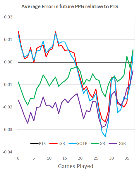
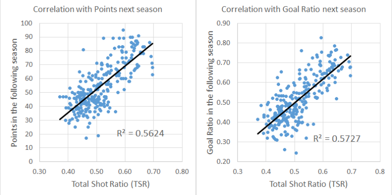
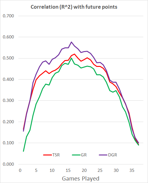
Let’s start with a very basic model, the Total Shot Ratio (TSR) from the last 5 games. This is calculated as Shots For / (Shots For + Shots Against), and gives a measure of how much teams are dominating games in terms of shots.

Step 1: Calculate the 5 game TSR for each team, using a few simple assumptions for teams new to the league who have fewer than 5 games.

Step 2: Use Excel’s SLOPE and INTERCEPT functions to convert the difference in TSR between the Home and Away teams into a predicted result for each game.

Step 3: Calculate the absolute error between the prediction and the result for each game.

Result: MAE =  1.276

Good news, that’s a decent improvement. However, I know from previous work that using data from 5 games isn’t really enough. To get a true measure of how good teams are, we need to look at a larger sample. A season is 38 games, and taking a rolling 38 game TSR reduces the MAE to 1.240.

Now, looking at shots is all well and good, but again in previous work I have shown that whilst shots are useful when we have limited data to play with, they are pretty poor when we have more than a few games worth of data.

For example, just using the number of Points won in the last 38 games produces a MAE of 1.236. A model that can’t predict better than points is a pretty poor model.

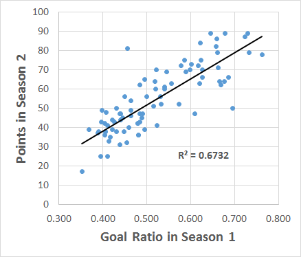
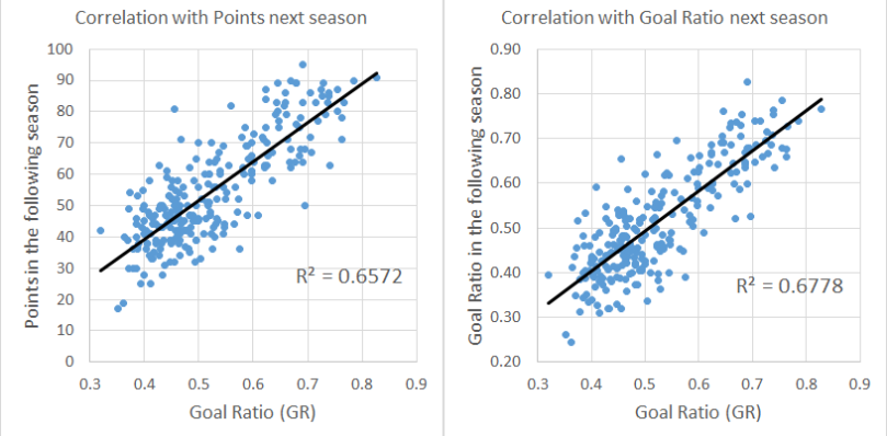
This is where Goals come into play. When we have enough data they are superior to just using shots, because we get an idea of how good the shots are, and how good the teams are at finishing/saving them.

Taking a 38 game Goal Ratio (GR), I get the MAE down to 1.234.

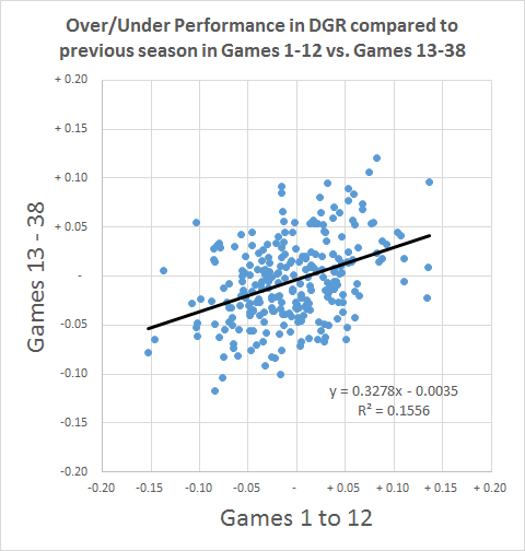
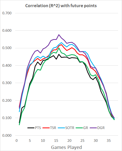
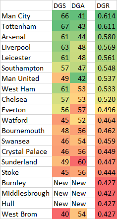
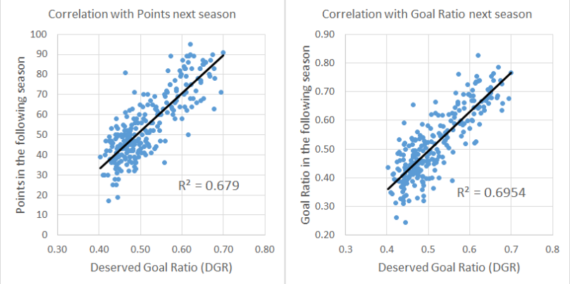
Last year I wrote a few blog posts about a Metric I called Deserved Goal Ratio (DGR), which uses a mix of shots and conversion rates regressed partly to the mean. Using this model improves results again, reducing MAE down to 1.228.

That’s as far as I could get with an individual model, but because different models have different weaknesses, we can often improve predictions by taking an average of different models.

To demonstrate how combining models can work:

38 Game TSR = 1.240
38 Game GR   = 1.234

Average of both models = 1.227

Taking an average of the 2 models produces less error than using either model individually, indicating that combining models is the way to go.

In order to combine models easily, I re-scaled each measure to be between 0 and 1, with 0 being the worst team on record and 1 being the best. Then I took an average of the measures from each model.

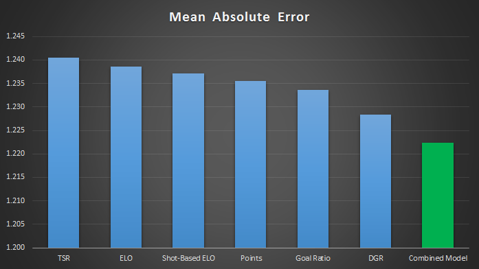
Combining 38 game TSR, GR, Points and DGR reduces the MAE to 1.224.

Another approach to rating teams is to use an ELO-based system, as used in chess and at Club-ELO. Building a simple ELO model where teams risk 4.6% of their points each game gave me a MAE of 1.239, which is worse than using Points.

However, this approach obviously has some advantages, as when combined with the above models the MAE reduced to 1.223.

Following the ELO theme, I built another model where teams risk 8.2% of their points, but the pot is divided in proportion to the shots taken in the match instead of being awarded to the winner. Again, individually the model was quite poor (MAE = 1.237), but when added to the mix the MAE reduced to 1.222.

My new model is therefore an average of the following:

38 Game Points
38 Game TSR
38 Game GR
38 Game DGR
Standard ELO
Shot-Based ELO

This model produces a Mean Absolute Error of 1.222 when predicting the score of an individual game.

An alternative measure of errors is RMSE, which penalises larger errors more. Which method is best is up for debate, but the Combined Model still comes out on top.

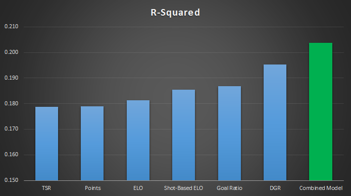
The Combined Model also performs best when using R-Squared, which measures the correlation between the match ratings and the results.

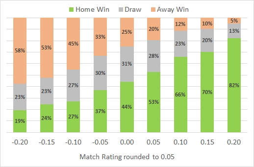
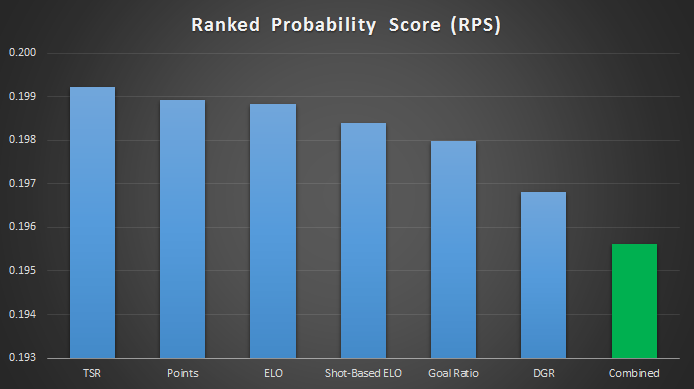
Alex B over at @fussbALEXperte has done some great work recently comparing various public models using a Ranked Probability Score (RPS), which uses the H/D/A probabilities to rate predictions. Using the RPS, the results look very similar.

All very good, I hear you cry. But how does this model compare to other public models?

Since Week 9 of this season, Alex has used the RPS measure to compare a number of models.

The RPS for my model for the first 120 games of this season is 0.1740, which I am told would rank among the top few models. However, 120 games is a small sample, so I will be interested to see how the model gets on for the remainder of the season.

Standard Deviation – A Comparison of Predictions

Note: At the time of publishing this post, 16 games have been played. As I began writing this last week when only 14 had been played, this post will ignore the most recent 2 games.

In my last post, I looked at the maximum standard deviation I would expect predictions to have at each stage of the season. In this post, I compare various public models and look at how they have changed over the season.

Unfortunately, there aren’t too many public models which make their weekly predictions easily accessible without trawling through months and months of twitter postings. Steve Jackson at @goalprojection helpfully puts his predictions on his website,  and Simon at @analytic_footy published his weekly predictions recently.

Comparing those 2 models to my own, here’s how the SDs have changed over the first 14 weeks of the season.

As before, the green line represents the maximum SD I would expect a model to have at each stage of the season. If a model goes above that green line, then there is either a problem with the methodology or the teams this season have a larger spread of ability than normal.

For what it’s worth, despite my model having the lowest SD as this point I’m still uncomfortable with it being that high. I don’t think that we can realistically claim to know enough about how well each team will do to justify such a high SD.

Whilst I haven’t yet collected together the weekly predictions, I know that @Goalimpact‘s model had much lower SD of around 4.5 a couple of weeks ago, which I think is probably more realistic.

Interestingly, @analytic_footy‘s predictions started out with the lowest SD, but increased sharply after week 2 and crept over the green line from about week 10. The SD after 14 games is very similar to what it was at the start of the season, meaning Simon expects there to be as much variance in just the next 24 games as he expected there to be in the whole 38 games at the start of the season. That’s a big change, which is because he believes there is a wider spread in team ability this year than average, which presumably wasn’t obvious at the start of the season.

 

In a future post, I want to look at whether that belief can be justified, and how easily we can predict the SD for games 14 to 38 based on data from the first 13 games.

Feedback is much appreciated. Also, if you have a model which you want adding to this post please let me know and I will update the graph.

Standard Deviation and Predicting the Premier League

Phil Birnbaum wrote a blog piece back in 2014 about how the spread of points in predictions should always be narrower than the spread of points in real life.

Put simply, this is because the spread of points is influenced by 2 factors:

1. The different abilities of the teams
2. Which teams get lucky or unlucky

We can’t predict which teams will be lucky, so we can only hope to predict the spread of points which is caused by their differing abilities. As this will be less than the total spread of points, predictions should always be narrower than real life.

“How much narrower?”, I hear you cry. Well, thankfully there is a mathematical equation which helps us to determine that.

SD(total)^2 = SD(ability)^2 + SD(luck)^2

SD stand for Standard Deviation, which is a mathematical measure of how spread out the points are. In Excel you can easily calculate the SD for a set of numbers using the STDEV() function.

As we are trying to calculate the SD attributable to ability, let’s rearrange this formula and start filling in what we know.

SD(ability) = SquareRoot ( SD(total)^2 – SD(luck)^2 )

First of all then, let’s look at the total spread of points. We can do this by looking at the SD of points scored in previous seasons.

So there’s quite a range, from 12.5 in 2010/11 to 19.7 in 2007/08.

On average, the total SD in a season is 16.7.

Let’s add that to our formula:

SD(ability) = SquareRoot ( 16.7^2 – SD(luck)^2 )

SD(ability) = SquareRoot ( 278.9 – SD(luck)^2 )

So, what about the luck? How do we start to calculate that?

Neil Charles estimated it here to be around 7.4.

Using the model I built for my previous posts on the natural limits of predictions (Part 1 and Part 2), I calculate a figure of 7.1. Using a model based on betting odds, I arrive at a figure of 7.4.

These models run lots of simulations of a league with a spread of ability similar to the premier league, using H/D/A percentages derived either from historical data or betting odds, and look at the range of points that can arise. As the abilities are the same in each simulation, any variation which emerges is entirely due to luck.

As these models all produce very similar figures, let’s take 7.4 and plug it into our formula.

SD(ability) = SquareRoot ( 278.9 – 7.4^2 )

SD(ability) = SquareRoot ( 278.9 – 54.8 )

SD(ability) = SquareRoot ( 224.1 )

SD(ability) = 15.0

Finally, an answer.

This means that for predictions made at the start of a season, 15.0 is the maximum SD we would expect to see, if a model had perfect knowledge of the ability of each team. Anything more than that is probably trying to predict which teams will be lucky, which is impossible.

The SD can be seen as a measure of confidence. A low SD is an acceptance that you can’t accurately measure the abilities of the teams. A high SD shows that you are confident about the accuracy of your model. If your SD breaks the maximum, there is probably something wrong with your methodology.

So, that’s all very good for pre-season predictions. But what about predictions part way through the season? We have had 13 games played already, what sort of SD should we expect for future points at this stage?

We can use the same method to calculate the maximum SD after each game, when predicting points scored in the remainder of the season. This produces the following:

The green line here represents the maximum SD we would expect a prediction to have at each stage in the season.

With 13 games played, the maximum SD value should be 9.9.

To calculate the SD of a prediction, we do the following:

1) Take the predicted final point tallies for each team
2) Deduct the number of points each team already has to get the predicted future points
3) Use the STDEV() formula on Excel on the predicted future points

To start with, let’s look at my own predictions:

Using the above method, I deduct points already scored from each week’s predictions, and then calculate the SD of the future points at each stage.

This results in the following:

Good news, my model has remained below the green line, which represents the average maximum predictable variance.

There are 2 reasons a model might go above the line:

1. There is a problem with the methodology
2. This season has a larger spread of points than average

In my next post I will look at other public models to see how they compare, and try establish whether this season has a larger spread of abilities than the average season.

Much of the above methodology comes from this post by James Grayson, whose blog is well worth a read.

As ever, feedback is much appreciated.

Why Leicester will (probably) finish in the top half

Leicester, the surprise champions of the league last season, currently find themselves down in 14th place after 12 games.

Last year, Leicester’s Deserved Goal Ratio (DGR) was 0.562, the 5th best in the league. With average luck, I would have expected this to translate into 65 points. In fact, they won 81 points, an over-performance of 25%.

Now DGR isn’t a perfect metric, and although it is better than other metrics at predicting performance there are elements of football that it doesn’t take into account. However, for the purpose of this blog let’s assume that DGR is a perfect way of measuring team skill.

Making this obviously incorrect but easy assumption, we can say that Leicester’s over-performance last season was sheer luck. Leicester should have got 65 points and finished 5th, but they got lucky and managed to win the league.

Based on this, coming into this season all I could do was expect Leicester to have average luck and win points in relation to their underlying skill. As most teams regress towards the mean a little bit between seasons, I expected Leicester to achieve around 63 points in 2016/17.

Assuming they won these points evenly over the season, after 12 games I would have expected them to have roughly 20 points. In fact, they have only 12.

Theory 1: They are still the same Leicester as last year

Maybe they have just been unlucky so far, and they are just as good as last season. If we expect them to have average luck from now on, they would achieve a score of 55 points, having already dropped 8 points from their expected total.

Theory 1 Prediction: 55 points.

Theory 2: They are much worse than last year

Maybe they haven’t scored many points because their performance has been genuinely poor this season. Let’s assume this season’s stats are representative of their new true level of ability.

So far this season, Leicester’s stats per game are as follows (previous season in brackets):

Shots for: 10.58 (13.76)
Goals for: 1.17 (1.79)
Conversion rate for: 11.0% (13.0%)

Shots against: 14.08 (13.58)
Goals against: 1.67 (0.95)
Conversion rate against: 11.8% (6.98%)

Deserved Goals for: 1.19 (1.58)
Deserved Goals against: 1.53 (1.22)
DGR: 0.437 (0.562)

The first thing to note is that Leicester’s underlying stats have all got worse compared to last season. They are taking fewer shots, and converting fewer of these shots into goals. Also, their opponents are taking more shots, more of which are going into Leicester’s net.

A DGR of 0.437 translates to 27 points in the rest of the season, which when added to the 12 they already have gives them a final total of 39 points.

Theory 2 Prediction: 39 points

Looking at the data

Before we can make this gloomy conclusion we need to look at whether a team’s performance after 12 games is a good indicator that a team’s ability has changed. If it is, we should expect the over/under performance so far compared to last season to continue in games 3-38.

Newsflash: It doesn’t.

OK, so it does to some extent. But it’s not a very strong relationship, and on average the over/under performance after 12 games falls away by about two thirds in the remainder of the season.

This is good news for Leicester. Their under performance so far of 0.125 DGR should reduce to an under performance of 0.044 DGR in games 13 to 38.

Our best guess of Leicester’s actual DGR for the remainder of the season is therefore 0.518 (0.562 – 0.044). This translates to 38 points in the rest of the season, meaning my best prediction is a final total of 50 points.

In summary then:

Original pre-season prediction: 63 points

Theory 1; Optimistic: 55 points

Theory 2; Pessimistic: 39 points

Looking at the data: 50 points

Nobody really expected Leicester to repeat last season’s result, as they over performed their underlying stats in a way that probably wasn’t sustainable. Their terrible start this season is evidence of a slight decline, but based on historical trends we should expect their stats to pick up quite a bit in the rest of the season. They won’t be winning the league, but they shouldn’t be anywhere near relegation either.

Of course, when predicting points you also need to consider the strength of the other teams in the league. My weekly predictions on Twitter do this, and at the moment I have Leicester predicted to win 52 points, and finish 9th.

Feedback is appreciated.

 

Testing Predictive Metrics for the Premier League

In this blog I look in detail at the predictive power of various metrics in the Premier League, to see which is best at predicting future performance at each stage of the season.

The metrics I am testing are as follows:

PTS = Points scored
TSR = Total Shot Ratio
SOTR = Shots on Target Ratio
GR = Goal Ratio
DGR = Deserved Goals Ratio

Test 1

For the first test, I want to imagine that we know nothing about each team at the start of the season.

Using data from the last 15 seasons, I will see how well each metric predicts points scored in the remaining fixtures. For example, after 10 games played I will see how well the metrics for the first 10 games predict points scored in games 11 to 38.

Note: To be consistent with a test I will perform later in the post, I am just looking at the 17 teams in each season who played in the season before. That means that the sample is 17*15, so 255 full seasons.

There are 2 methods of testing predictive power. The first is looking at the correlation (R^2), and the second is looking at the average errors (MAE). Let’s start with correlation, where higher numbers are better.

So, if we don’t know anything about the teams at the start of the season, this test would indicate that we should use DGR for the majority of the season, although SOTR takes the lead briefly between 26 and 29 games played. TSR is slightly worse than SOTR pretty much all season, and PTS and GR start off badly and never catch up with the rest.

Whilst using R^2 to test predictive power is widespread, a better test is to look at the average error per game when using each metric to predict future points.

To make the graph easier to interpret, I have shown the results relative to the results for PTS. On this graph, low is good.

We can see from this that the average errors agree with the R^2 results. DGR still dominates for most of the season, SOTR takes the lead for a brief period etc.

 

However, there is a problem with this approach. We don’t start the season knowing nothing about the teams.

Goal Ratio gets a bad result in the above test, but as examined in a previous post we know that GR in one season correlates more with points in the following season than TSR, so it must have some decent predictive power with a larger sample.

Test 2

Let’s repeat the above test, but instead of assuming we know nothing at the start of the season, let’s be more realistic and start off with the previous season’s data, and then use a 38-game rolling score as the teams progress through the season.

Here’s the R^2 results, with our previous results greyed out for comparison. High is good.

Obviously, our early season results are much better. In addition, the previously poor GR redeems itself, being a better early season predictor than both shot-based metrics, which fall behind PTS in the same period. DGR still dominates, and SOTR still takes a brief lead later on. Importantly, almost all these results are better than just using in-season data.

Again, I’ve done the average errors test relative to the results for PTS. Low is good.

Once more, this tells a similar story to the R^2 values. DGR takes an early lead over GR, and is overtaken by SOTR for a brief period. The later stages of the season are a mix of DGR and the shot-based metrics.

In summary then, DGR is the best early-season predictor, both when limited to in-season data and when using data from the previous season. SOTR is a good metric for the later stages, although DGR does well here too. GR is a strong metric, but only worth using with access to results from the previous season, as it takes too long to pick up a signal within a season.

Full results are available on google sheets here: Google Sheets Results.

To finish off, what does this mean for the current season?

Well, with 6 games played, a rolling 38 game Deserved Goals Ratio has a higher correlation and lower average error than any other metric tested here. If you can’t be bothered to calculate that, a rolling 38 game Goal Ratio is not far behind.

If you insist on only looking at this season, DGR is still the best after 6 games, followed by Shots on Target Ratio. However, these in-season metrics are significantly worse than longer-term approaches, so it’s worth the time looking a bit further back for information about the relative strength of the teams.

As an example, Points scored in the first 6 games correlates with points scored in games 7-38 with an r^2 of 0.329, and an average error of 0.296.

38-game DGR after the first 6 games correlates with an r^2 of 0.670, and an average error of 0.202.

Follow me on Twitter @8Yards8Feet

The idea for these graphs comes from 11tegen11, whose blog is well worth a read.

The Natural Limits of Predictions (Part 2)

In my last post, I calculated a value of 6.5 points as the minimum average absolute error a model can reliably achieve when predicting a season’s worth of points for each team in the Premier League.

However, this was based on a simple simulation of a league full of evenly matched teams, with an adjustment for home advantage. It is therefore not particularly accurate, as not all teams are equally matched.

To simulate more realistically, we need a representative spread of the abilities of the teams. As a proxy for this, I have taken the average points scored by position over the last 16 seasons, on the assumption that this will produce a fairly accurate distribution of the teams’ abilities.

Previously, we used the average Home/Draw/Away percentages and applied them to an average team. This time, we need to adjust these percentages based on the relative strength of teams in each fixture.

Looking at historic results, we can see the relationship between final points in a season, and individual results within that season. Based on this, we can calculate formulas which convert the relative strength of 2 teams into Home/Draw/Away percentages for individual matches.

We can then run a simulation of a full 38 game season, with the probabilities for each match being calculated using the above formulas.

If we run this simulation many times, we get a large sample of simulated points, and we can take an average of the variance from the mean for each team.

After 25,000 simulations, the average variance from the mean was 5.7 points.

This means we can adjust our figure from 6.5 points to 5.7 points. In the Premier League, 5.7 points is the lowest average absolute error in points we could consistently achieve with pre-season predictions.

Another interesting thing to note is how the average variance differs depending on how good a team is.

It looks like it’s easier to accurately predict the best and worst teams, but more difficult to predict the middle of the table.

In summary, an average absolute error of 5.7 points is the natural limit for Premier League predictions, and you should expect bigger errors in the middle of the table than at the top and bottom.

The Natural Limits of Predictions (Part 1)

Let’s say we want to predict the points scored for each team in a Premier League season.

You might think that a perfect model would predict the points exactly right. However, that’s impossible to do consistently because of a mixture of random and chaotic variation, which introduces an element of unpredictability into every model. Because we can never perfectly measure the current skill of the teams, we can never perfectly predict their skill over the season. Also, we don’t know which teams will get lucky or unlucky.

When we make predictions using statistics we assign values to each team, which we think represents their current skill level. This could be as simple as Goal Difference in the previous season, or as complicated as an Expected Goals model. In any case, the outcome is a set of “skill values”.

These skill values are a product of past performance, intended to measure the current ability of the teams, and we make the assumption that a team’s performance in the future will be roughly the same as its performance in the past.

We know that football results are a mixture of skill and luck. Over a Premier League season of 38 games for each team luck will mostly cancel out, meaning we can be fairly confident that accurately describing the skill of each team will produce decent predictions.

This produces nice charts like this which show a decent correlation between performance in one season and points in the next season. This chart looked a lot nicer before last season, when Leicester and Chelsea added the 2 obvious outliers.

Some of the variation between seasons is down to genuine changes in ability, but even over a full season luck still plays a part. We can show this by simulating a Premier League season of 38 games for an average team.

There are 3 outcomes in a Football match. Win (3 points), Draw (1 point) and Loss (0 points).

These outcomes are not all equally likely for an average team. Draws don’t happen as often as Home and Away wins, and there is a noticeable home advantage.

Using data from previous seasons, we can generate probabilities for each outcome. We can then run a Monte Carlo simulation to see how many points our average team is expected to achieve over the season.

For 19 “Home games”,  we will use 46.3% chance of a win, and 25.8% chance of a draw. For 19 “Away games”, we will use 27.9% chance of a win, and 25.8% chance of a draw.

The results from 5000 simulations are as follows:

These results return an average points score of 52.1, which encouragingly matches the actual average points scored in the last 16 Premier League seasons. However, there is plenty of variation around that central result.

The average variation from the mean was 6.5 points. 

This means that even if we had a brilliant metric which described the relative skill of each team near-perfectly at the start of the season, we would still expect to see an average error of 6.5 points between our pre-season predictions and the actual results.

We could therefore conclude that 6.5 points is our “Holy Grail” for the Premier League. Theoretically, no predictive metric could ever consistently achieve a lower average error than this.

However, this is all based on an average team playing a season against other average teams. In reality, some teams are better than others, and it may be easier to predict the points for games between teams of varying abilities.

I develop the method further in Part 2.

 

As always, feedback is very welcome.

All data is from http://www.football-data.co.uk/

Follow me on twitter @8Yards8Feet

Deserved Goals: Predicting the 2016/17 Season

In my last post, I introduced a metric called Deserved Goals Ratio (DGR) for predicting future performance. In this post I use it to predict the 2016/17 season.

For each game in our sample of the last 16 Premier League seasons, we calculate the Deserved Goals Ratio for each team, based on their 38 most recent matches. Taking the Away Team’s ratio away from the Home Team’s ratio gives us a “match rating”.

For example, when Leicester played Everton on 7th May 2016, the calculation was as follows:

Leicester: Deserved Goals For: 61, Deserved Goals Against: 47
DGR = 0.56

Everton: Deserved Goals For: 55, Deserved Goals Against: 55
DGR = 0.50

Match Rating = 0.56 – 0.50 = 0.06

If we repeat this calculation for every game over our sample, we can see how match ratings relate to results:

Using Excel’s SLOPE and INTERCEPT functions, we can produce formulas to work out the chances of a Home Win, a Draw or an Away Win for a given match rating.

Home Win % = Match Rating x 1.62 +0.46
Draw % = Match Rating x -0.17 + 0.26
Away Win % = Match Rating x -1.45 + 0.28

For the Leicester vs. Everton example used above, the match rating of 0.06 produces the following probabilities:

To predict the 2016/17 season, we calculate the DGR for each team, based on their performance in 2015/16. As 3 teams from last year were relegated, we do not have data for the 3 newly promoted teams, namely Burnley, Middlesbrough and Hull City. The average score for the league should be 0.5, so these 3 teams are all given the same score in order to arrive at this average.

As above, we calculate the match rating and the probabilities for each game. Using a Monte Carlo simulation (which sounds complicated, but just means using random numbers to generate outcomes in proportion to the calculated probabilities for each match), we can see how many points we expect each team to score.

Running 5000 simulations produced the following result, the bars representing the central 90% of the simulations.

Using the results of the simulations, we can predict how likely it is that each team wins the league.

So Deserved Goals expects the title race to be a close fight between Man City and Tottenham, with Man City just having the edge.

A New Metric – Deserved Goals

In a given season of 38 games, we can break down goals scored as follows:

Goals Scored = Shots x Conversion %

Both of these components have an element of skill and an element of luck.

Goals Scored = (Deserved Shots + Effect of luck) x (Deserved Conversion % + Effect of luck)

The effect of luck can be positive or negative, depending on whether a team was lucky or unlucky.

We can add some numbers to this formula, based on statistics from the last 16 Premier League seasons from which we can calculate average shot and conversion rates. We can also calculate how much of the variance from the average is attributable to luck, by calculating how much they regress to the mean between seasons.

What we know:

Average shots taken per season = 453
Average conversion rate = 11.09%
Shots taken above or below average = 80% skill, 20% luck
Shots against above or below average = 81% skill, 19% luck
Conversion % above or below average = 46% skill, 54% luck
Save % above or below average = 40% skill, 60% luck

Adding in those numbers to our formula produces the following:

Goals Scored = (453 + 80% x (Shots – 453) + 20% x (Shots – 453)) x (11.09% + 46% x (Conversion % – 11.09%) + 54% x (Conversion % – 11.09%))

When producing a metric we can use to predict future performance, we cannot predict future luck. We therefore only want to measure the goals produced due to skill, i.e. the Deserved goals.

This is the problem with traditional Goal Ratio, as it includes the luck element along with the skill. Total Shot Ratio is similarly flawed, as it includes the luck in terms of producing shots, and removes finishing skill by assuming a constant conversion rate.

Removing the luck element produces the following formula:

Deserved Goals Scored (DGS) = Deserved Shots x Deserved Conversion %

Or with numbers:

DGS = (453 + 80% x (Shots – 453)) x (11.09% + 46% x (Conversion % – 11.09%))

Using the same method for Deserved Goals Against (DGA), we produce the following:

DGA = (453 + 81% x (Shots – 453)) x (11.09% + 40% x (Conversion % – 11.09%))

We can then produce a Deserved Goals Ratio (DGR) metric, as follows:

Deserved Goals Ratio = DGS / (DGS + DGA)

As this only includes the skill element of shots and conversion %, this metric should be better at predicting future performance than traditional GR or TSR, both of which include past luck and try to use it to predict future skill.

We can test this by looking at how well the metrics for one season correlate with points scored and goal ratio achieved in the following season.

All data is from the last 16 Premier League seasons.

Deserved Goal Ratio (DGR)

Total Shot Ratio (TSR)

Goal Ratio (GR)

Conclusion: DGR is better at predicting next season’s performance than GR or TSR.

We can also test within a season, to see how well the metrics so far predict future points at each stage in the season.

Conclusion: DGR is better at predicting future performance within a season than GR or TSR.

Feedback is much appreciated.

Follow me on Twitter here.

Many thanks go to the work of James W Grayson, 11tegen11 and FootballData.