Snooker through the Ages – 1986/87

The 1986/87 season had a total of 145 players, up from 128 the previous year.

There were 93 active players, and their final ratings based solely on their performances in this season were as follows:

Once again, Steve Davis was top of the pile. He began the season with a run to the Final of the 1986 Australian Masters, losing 3-2 to Dennis Taylor. A loss in the Semi Final of the 1986 Thailand Masters to James Wattana followed, before he won his first tournament win of the season at the 1986 China Masters. Two Semi-Final defeats followed, at the 1986 Malaysian Masters and the 1986 Hong Kong Masters. He did one better at the 1986 Matchroom Trophy, reaching the final but losing out to Willie Thorne 10-9.

Davis was upset by Eugene Hughes in the Quarter Final of the 1986 International Open, and lost out to Rex Williams in the Quarter Final of the 1986 Grand Prix. Better form was found at the 1986 Canadian Masters, where Davis beat Willie Thorne 9-3 in the Final to win the event. Another win soon followed, as Davis won the 1986 UK Championship, before once again losing out at the single-frame Pot Black event. Long format snooker continued to bring more success, Davis winning the Final of the 1987 Classic 13-12 against Jimmy White.

He could not get past the Last 16 of the 1987 Masters, or the Last 32 of the 1987 British Open. He then lost out in the Semi Final of the 1987 Kent Cup, before winning the 1987 Irish Masters, defeating Willie Thorne 9-1 in the Final. Another win followed at the 1987 Matchroom League, where Davis topped the table.

Davis reached the 1987 World Championships with a point to prove, having lost in the Final for 2 consecutive years. This time, there was to be no upset. Warren King made it interesting, but was overcome 10-7. Ray Reardon, now way past his best, was beaten 13-4. Terry Griffiths was beaten 13-5, then Jimmy White 16-11.

The Final was a repeat of the year before, as Joe Johnson had once again managed to reach the last stage against long odds. This time, there was to be no miracle victory, and Steve Davis reclaimed his World Title. He was the #1 Player in the World, and now a 4-times World Champion.

Snooker through the Ages – 1985/86

The 1985/86 season had a total of 128 players, up from 119 the previous year.

There were 87 active players, and their final ratings based solely on their performances in this season were as follows:

Steve Davis held onto the #1 position for the 6th consecutive year. He began the season by winning the 1985 Singapore Masters, before losing in the group stage of the 1985 Thailand Masters. He reached the Final of the 1985 Hong Kong Masters, losing to Terry Griffiths, then lost in the Quarter Final of the 1985 Matchroom Trophy to Jimmy White. Next up was the 1985 Grand Prix, which Davis won, beating Dennis Taylor 10-9 in the final. This result was reversed in the following month, when he lost to Taylor 9-5 in the Final of the 1985 Canadian Masters. Davis lost 1-0 in the Quarter Final of Pot Black, but won yet another major title at the 1985 UK Championships, beating Willie Thorne 16-14 in the final. Another clash with Dennis Taylor followed in the Final of the 1985 KitKat Break for World Champions, this time Davis losing 9-5.

The new year would start with a Quarter Final defeat to Jimmy White at the 1986 Classic, and another Quarter Final defeat to Terry Griffiths at the 1986 Belgian Classic. He did one better at the 1986 Masters, reaching the Semi Final before losing once more to Jimmy White. His quest for a title in 1986 would continue as he crashed out of the English Professional Championship to Tony Meo in the Semi Final, before finding success at the 1986 British Open, with a victory of 12-7 over Willie Thorne in the Final.

The World Championships were next, and once again Steve Davis started strongly. Ray Edmonds was beaten 10-4, then Doug Mountjoy 13-5. Jimmy White was beaten 13-5, then a 16-12 win over Cliff Thorburn put Davis into another World Final. However, as in the previous year, Davis would fall at the last hurdle.

If you were a betting man, you could have made good money on Joe Johnson, who entered the World Championships as a 150/1 underdog. He had never won a tournament, never won a match in 3 attempts at the World Championships, was the 16th seed, and had ranked 24th in my rankings the previous season. He started the season with a loss in the Quarter Final of the 1985 Australian Masters, and did the same in the 1985 Matchroom Trophy. He lost in the Last 16 of the 1985 Grand Prix, the Last 32 of the 1985 UK Championship, the Quarter Final of the 1986 Classic, the Last 16 of the 1986 Masters, the Quarter Final of the 1986 English Professional Championship and the Last 32 of the 1986 British Open. It is fair to say that Joe Johnson was not a serial winner.

Johnson started the World Championships with a 10-3 win over Dave Martin. This was expected, with Martin being a lower ranked player, but it was a sign of things to come as Johnson went on to defeat Mike Hallett 13-6, who had just beaten defending champion Dennis Taylor. This set up a Quarter Final clash with #8 seed Terry Griffiths. Johnson was losing 12-9, but won the last 3 frames to win 13-12, and reach the Semi Final. Tony Knowles was the #4 seed, but Johnson never looked like losing, winning 16-8 and reaching the World Final.

Davis and Johnson met in the final, with Davis a heavy favourite. The match started as a close affair, and the score was tied at 8-8 after the first day, but Johnson then pulled ahead and eventually won 18-12 to become World Champion. He climbed to #8 in my rankings, with Davis still being the dominant player, but not having won the world title since 1984.

Snooker through the Ages – 1984/85

The 1984/85 season had a total of 119 players, up from 102 the previous year.

There were 74 active players, and their final ratings based solely on their performances in this season were as follows:

Steve Davis was once again #1, but the gap between him and the chasing pack closed. Davis started his season with 3 group-format tournaments, and finished as runner up in the 1984 Singapore Masters, before coming third in the 1984 Malaysian Masters and last in the 1984 Thailand Masters. A return to Knockout tournaments found more success, winning the 1984 Hong Kong Masters, the 1984 Scottish Masters and the 1984 International Open in succession. The 1984 Grand Prix saw him lose in the Semi Final to Cliff Thorburn, but he bounced straight back at the 1984 UK Championship, beating Alex Higgins 16-8 in the final. The new year saw Davis lose in the semi final of the 1985 Classic, and the last 16 of the 1985 Masters, before he won the 1985 English Professional Championship in February. The 1985 British Open saw him lose in the Semi Final, as did the 1985 Irish Masters. Entering the World Championship then, Davis was favourite, and reached the final without too much difficulty. However, this wasn’t to be his year.

Dennis Taylor had established himself as the closest rival to Davis. Ranked #2 by me in the previous season, he had built on his success. During the season he had won the 1984 Costa Del Sol Classic, the 1984 Grand Prix and the 1985 Irish Professional Championship. At the World Championships, he beat Silvino Francisco 10-2, Eddie Charlton 13-6, and Cliff Thorburn 13-5, in a tactical battle where only 1 half-century was scored in 18 frames. He beat Tony Knowles 16-5 in the Semi Final, setting up a meeting with Davis in the Final. What followed is probably the most famous match in snooker history, where Taylor was trailing for the entire match before winning a decider on the black ball in the deciding frame. Steve Davis was still the #1 player, but Dennis Taylor was the new world champion.

Snooker through the Ages – 1983/84

The 1983/84 season had a total of 102 players, up from 77 the previous year.

There were 62 active players, and their final ratings based solely on their performances in this season were as follows:

For the 4th consecutive year, Steve Davis tops the pile. He started the season with a 3-0 loss in the 1983 Hong Kong Masters to Doug Mountjoy, which he avenged 2-1 in the 1983 Thailand Masters before losing in the final. He won his first title at the 1983 Scottish Masters, followed by winning the 1983 International Open.

He lost in the last 32 of the 1983 Professional Players Tournament, then had a run to the final of the 1983 UK Championship where he narrowly lost to Alex Higgins 16-15 in the final. At the turn of the year, he lost in the Quarter Final of the 1984 Pot Black but then won the 1984 Classic. Defeat in the quarter final of the 1984 Masters to Kirk Stevens was a setback, but he then won the 1984 Tolly Cobbold Classic in February, beating Stevens en route to the title.

Another victory followed in the 1984 International Masters, followed by another in the 1984 Irish Masters, meaning Davis arrived at the Crucible having won 3 straight tournaments.

The World Championships was a familiar story for Davis. 10-3 over Warren King in the first round, then 13-5 over John Spencer in the second. The Quarter Final against Terry Griffiths was 13-10, then the Semi Final was a 16-9 win over Dennis Taylor. The final was between Davis and Jimmy White, who had reached his first World final. Davis took an early lead, but White fought back and made it a close result in the end. Davis won 18-16 to win his third World Title and cement his place as one of the great players.

Snooker through the Ages – 1982/83

The 1982/83 season had a total of 77 players, up from 73 the previous year.

There were 34 active players, and their final ratings based solely on their performances in this season were as follows:

Steve Davis continued his dominance. He started the season by winning the 1982 Australian Masters in August, followed swiftly in September by winning the 1982 Scottish Masters, beating Alex Higgins 9-4 in the final. He faltered in the 1982 International Open, losing in the Quarter Final to David Taylor, and similarly lost to Terry Griffiths at the same stage in the 1982 UK Championship.

He returned to winning ways at the turn of the year, winning the 1983 Pot Black, and the 1983 Classic in January. He lost in the 1983 Masters Quarter Final, then made up for this by winning the 1983 Tolly Cobbold Classic. He did not progress past the Semi-Final group at the 1983 International Masters, but won the 1983 Irish Masters with an impressive 9-2 win over Ray Reardon.

The 1983 World Championships was a rout. Rex Williams was dispatched 10-4. Dennis Taylor put up a fight, but succumbed 13-11. Eddie Charlton was thrashed 13-5. Defending Champion Alex Higgins was destroyed 16-5. In the final, Cliff Thorburn was dominated 18-6. Steve Davis was back on top of the world, and there wasn’t any doubt about it.

Snooker through the Ages – 1981/82

The 1981/82 season had a total of 73 players, up from 63 the previous year.

There were 32 active players, and their final ratings based solely on their performances in this season were as follows:

The best player was Steve Davis, for the second season in a row. He had a blistering start to the season. He won the 1981 International Open, reached the semi final of the 1981 Scottish Masters, reached the final of the 1981 Northern Ireland Classic, won the 1981 UK Championship, won the 1982 Pot Black, reached the final of the 1982 Classic, won the 1982 Masters, won the 1982 Tolly Cobbold Classic, won the 1982 International Masters, reached the final of the 1982 Irish Masters, then reached the semi-final of the 1982 Highland Masters.

It was no surprise, therefore, that he reached the 1982 World Championships as a huge favourite to defend his title. However, he crashed out in a shock 10-1 loss to Tony Knowles in the first round. In a reversal from the previous season, he won the final event of the season, the 1982 Pontins Professional, finishing a massively successful season with a win, and the number 1 spot with a score of 1212. The world title, however, had eluded him.

To say that Alex Higgins was an unlikely World Champion is an understatement. He entered the tournament as the #11 seed, 10 years after he last won the event. He had ranked 9th in my rankings the previous season, and in his own words was having the “worst season of my professional career”. He had failed to progress past the semi-finals in every major event, and excluding the World Championships had lost more frames than he had won across the season. At the Crucible, he started with a relatively easy draw against Jim Meadowcroft, who he beat 10-5. He then faced a tougher opponent in the form of Doug Mountjoy, and squeaked through 13-12 in a decider.

Progressing to the quarter finals, he played Willie Thorne, beating him 13-10. In the semi-final he faced a young Jimmy White, and was trailing 15-13 when he made 3 successive half-centuries to win 16-15. His break to level the match was a potting masterclass, where the white ball was rarely under control but he managed to pot his way out of trouble and clear the table. The World Final against Ray Reardon was another close game, and stood at 15-15 before Higgins found his form and won 3 successive frames to win the title for a second time.

This win helped Higgins maintain a good rating of 1039, but due to the improvement of other players he fell from 5th to 6th in my rankings. He was, however, World Champion once again.

Snooker through the Ages – 1980/81

The 1980/81 season had a total of 63 players. To be listed in my rankings, players must be “active”, which I define as having either played at least 10 matches, or having reached the semi-finals of the World Championships. However, all players are included when calculating the player ratings.

There were 19 active players, and their final ratings based solely on their performances in this season were as follows:

The best player was Steve Davis. He started the season relatively poorly, losing 9-2 to Terry Griffiths in the quarter final of the 1980 Canadian Open in August, then failing to win his group in the 1980 Champion Of Champions in October. His first tournament win of the season, and of his professional career, came in the 1980 UK Championship, where he beat Tony Meo 9-5, Terry Griffiths 9-0 and Alex Higgins 16-6 to win the November event. He followed up on this in the following month by winning the 1980 Classic, with wins over Cliff Thorburn, David Taylor and Dennis Taylor.

A bad spell followed. He was out of luck in the single-frame 1981 Pot Black event, losing all his matches, and lost 5-3 to Perrie Mans in the first round of the Masters. He did not participate in the 1981 Tolly Cobbold Classic, and lost 4-2 to Ray Reardon in the Quarter Final of the 1981 Irish Masters.

In March, Davis found his form, winning the 1981 Yamaha Organs Trophy and the 1981 English Professional Championship in quick succession. He carried this good form into April, and went into the World Championships as the favourite with the bookies, despite being seeded 13th.

In Sheffield, he met Jimmy White in the first round, winning 10-8. He met Alex Higgins in the second round, winning 13-8. In the quarter final he played Terry Griffiths, winning 13-9. The semi final was against the reigning champion and number 1 seed Cliff Thorburn. In a bad tempered match, during which Thorburn took umbrage at Davis’ offered handshake when 57 ahead with the pink and black still remaining, David emerged victorious 16-10. The final was against Doug Mountjoy, also in his first World Final. David took an early lead, and stayed ahead throughout, emerging as World Champion with an 18-12 victory.

A first round loss to Terry Griffiths in the 1981 Pontins Professional was of little importance after the win at the Crucible, and he finished the season as the #1 player in the world, with a rating of 1212.

Snooker through the Ages – Introduction

I have developed a method of ranking snooker players, which I will attempt to explain here. I will then write a series of posts which cover the long history of snooker, ranking players each season and comparing players over time.

No method is perfect, and my method isn’t either. Nevertheless, the results do seem to make sense, and I hope it is as interesting to read about as it was to develop.

The starting point is the basis of most rating systems, which is that every player has a score denoting their skill level. The difference in scores between 2 players can be converted into a chance of winning a given match. I have used the same scale as used by the Elo system, where a player with a 200 point advantage should win around 75% of their frames, and a player with a 400 point advantage should win around 90%.

For the purposes of this exercise, I assume that every player has a fixed rating for any given season, which does not change during the year.

The method I have used is as follows:

Let’s take a best of 19 match between 2 players. We don’t know anything about their abilities yet, so let’s assume they both have a rating of 1000.

If Player 1 wins the match 10-4, he has won 71% of the frames played. Given the scale I have used, we would expect a player to win 71% of frames against a player with 159 fewer points.

We can therefore approximate the ratings of the 2 players, by placing them 159 points apart, with the midpoint being the average of their previously estimated scores (1000).

That gives us estimated ratings of Player 1 (1079.50) and Player 2 (920.50).

As the lengths of snooker matches vary, I give these estimated ratings a weighting based on the length of the match, with best-of-19 or above having a weighting of 1, best of 3 being 3/19^ths, best of 5 being 5/19^ths, etc.

If this calculation is done for every match in a season, and the weighted average is taken for each player, we have an estimated rating for each player.

Of course, these ratings are not great. Because we started assuming every player had a rating of 1000, the initial output is better than nothing, but fairly naïve as it doesn’t reward wins over good opponents or punish losses to weaker players.

Thankfully, we can repeat the process, but instead of using 1000 as the inputs, we use the ratings we have just calculated. This then becomes an iterative process, with the output being fed back in over and over again until the ratings converge on a settled result.

We can see that the estimates are improving by calculating the difference between the ratings and the estimated ratings for each match, taking a weighted average, and seeing this reduce with each iteration of the system. Eventually, the error stops reducing. At this point, the error has been minimised, and we have our final ratings for each player in that season.

In themselves, these ratings are only useful in a relative sense, in that the differences between players tell us something, but a rating of 1300 doesn’t really mean anything.

Ideally, we will have a standard against which all ratings can be judged. In my method, I have moved all the ratings in the 1980-81 season, so that the average of the top 16 players is 1000.

In all other seasons, I have first calculated the difference between all the players, and then placed these on the scale in such a way that the differences between the ratings of established players in successive seasons is minimised. This allows all ratings in all years to be seen on the same scale.

In my next post, I will review the 1980-81 snooker season, and calculate the ratings for that year.

UPDATE:

Having reviewed the rankings produced by the above method, I have made 2 changes.

Firstly, the weighting for the estimated ratings now include a preference for players with more matches played, so it is not as easy to get a high rating by beating players with few matches.

Secondly, snooker players play to win matches, not just to maximise frames won. To account for this, if a player wins 60% of his frames, I will give a score of 80% (The average of 100% for a win, and 60% for the frames won). If a player wins 20% of his frames, I will give him a score of 10% (The average of 0% for a loss, and 20% for the frames won).

I find this produces ratings which seem better than the initial version.

Deserved Goals 2.1

In my last post (which I recommend you read before this), I improved my original Deserved Goals model, which resulted in the following formula:

Deserved Goals 2.0 = (( Average Shots+ A% of the variance ) x ( Average Combined xG per Shot + B% of the variance )) x ( Average Goals per Combined xG + C% of the variance )

I estimated figures for A, B and C, and showed that in-sample, it performed well against other metrics at predicting the Premier League.

However, there are a number of issues with this approach. Firstly, to properly test a metric it is important to separate your data into “training” and “testing”. You should only use the training data to develop the metric, and then you should test it on the unseen testing data to see how it performs. Also, a metric should be able to perform well in other top leagues, not just the Premier League.

I have therefore widened the scope to encompass the top 5 European leagues (England, Spain, Germany, France and Italy), and split the data as follows:

Training Data: 2016/17 & 2017/18, a total of 3652 games

Testing Data: 2018/19, a total of 1,826 games

Ignoring the testing data for now, I will develop the metric using only information from the training data.

To do this I need to find values for the following variables. These need to work well in the training data, have some basis in theory, and be general enough to avoid over-fitting.

Deserved Goals = (( Average Shots+ A% of the variance ) x ( Average Combined xG per Shot + B% of the variance )) x ( Average Goals per Shot Based xG + C% of the variance )

Let’s work through these one at a time.

Average Shots is easy, as we can just see what the average number of shots taken by a team was in our training data. There were 90,858 shots taken in 3,652 games, with 2 teams in each game, which is 12.4 shots per game per team.

Average Combined xG per Shot should theoretically be the same as the average conversion rate (assuming xG accurately reflects the chance of a goal being scored). In the training data, there were 10,121 goals scored from 90,858 shots, which is a conversion rate of 11.1%.

Average Goals per Shot Based xG should theoretically be 100%, again assuming xG is a good measure of the chance of a goal being scored.

Filling in those figures gives the following:

Deserved Goals = (( 12.4 + A% of the variance in shots) x ( 11.1% + B% of the variance in Combined xG per Shot )) x ( 100% + C% of the variance in Goals per xG)

As for A, B and C, we need to look at how these 3 components regress to the mean within a season. Again, we will only use the training data.

Let’s start with Shots. In the charts below, on the left is the correlation between the shot rate at each stage in the season, and the shot rate in future games, for both Shots For and Shots Against. We can see that Shots For are more repeatable, indicating that taking shots is more of a skill than not allowing your opponent to take shots. This tells me that to get better predictions, I need to have different input values for Attack and Defence.

The other thing to notice is that the data is noisy. This reflects what actually happened in the training data, but if we want it to actually tell us something about football we need to look at the trend.

The right hand side shows the trend I will use in my metric. For the first half of the season (19 games), I have plotted a logarithmic trend line. I have then fixed the value at the value after 19 games for the remainder of the season. This is because I believe the drop off in correlation reflects the diminishing number of games remaining, not an actual drop off in predictive power.

Put simply then, the value for A will vary depending on how many games have been played. This is because after a few games we are much less sure that the variation reflects ability rather than luck than we are after a larger number of games.

Repeating this for the other components produces these results, which will be the inputs for A, B and C.

For all 3 components, it seems like it is easier to rate Attack than Defence. Using these values should improve predictions, as we will regress defensive statistics towards the mean more than the attacking statistics.

OK, so this is the new form of the metric (v2.1), which uses the figures we calculated and the inputs from the above chart:

Deserved Goals For = (( 12.4 + A% of the variance in shots for) x ( 11.1% + B% of the variance in Combined xG per Shot for)) x ( 100% + C% of the variance in Goals per xG for)

Deserved Goals Against= (( 12.4 + A% of the variance in shots against) x ( 11.1% + B% of the variance in Combined xG per Shot against)) x ( 100% + C% of the variance in Goals per xG against)

Deserved Goals Ratio = Deserved Goals For / (Deserved Goals For + Deserved Goals Against)

Now we have a metric, it’s time to work out the relationship between the metric and future points, again only using the training data. Using the Slope and Intercept functions in Excel for each week of the season, and taking an average of results of the middle 11 games where the values should be more stable, I get the following formula:

Future Points per Game = (4.48 x Deserved Goals Ratio) – 0.88

As a quick sense check, the average team should have a ratio of around 0.500.

4.48 x 0.500 – 0.88 = 1.36 points per game

1.36 points per game over a 38 game season is around 52 points, which is about right for an average team.

OK, so we have arrived at a complete model. Here are the results for each metric within the training data:

As expected, the model does well within the training data. However, the real test is to see how it gets on with the testing data, which it hasn’t seen yet.

Here are the results with the testing data:

Whilst the difference is not as large as in the training data, Deserved Goals 2.1 still races into an early lead, and is the best overall metric.

Looking at correlation instead of average errors, we get a similar picture in the testing data:

This is an encouraging result, and shows that Deserved Goals 2.1 would be a good metric to choose when trying to predict future performance in top level club football.

If you have any questions, comments or suggestions, please let me know. I am on Twitter @8Yards8Feet

Data from: http://www.football-data.co.uk/  and https://projects.fivethirtyeight.com/soccer-predictions/

Deserved Goals 2.0

Back in 2016, I introduced a new metric called Deserved Goals. This was an attempt to quantify the underlying skill of Premier League teams, and develop better predictions than the existing metrics.

I was pretty happy with it, and I have had some success using the metric to predict the Premier League, especially when combining it with other metrics. However, 3 years later I think I can make some improvements.

The original Deserved Goals used the number of shots taken by a team and their conversion rate of shots into goals, regressed towards the average. For shots taken, I kept 80% of the variance from the average, and for conversion rate I kept 46% of the variance.

Deserved Goals = ( Average Shots + 80% of the variance ) x ( Average Conversion + 46% of the variance )

I calculated 453 as being the average number of shots taken in a season, and 11.09% being the average conversion rate.

Deserved Goals = (453 + 80% x (Shots – 453)) x (11.09% + 46% x (Conversion Rate – 11.09%))

So a team which took 500 shots in a season and scored 70 goals, which is a 14% conversion rate, would have a Deserved Goals score of 61 goals.

Deserved Goals = (453 + 80% x (500-453)) x (11.09% + 46% x (14%-11.09%))

Deserved Goals = (453 + 80% x 47) x (11.09% + 46% x 2.91%)

Deserved Goals = (453 + 37.6) x (11.09% + 1.34%)

Deserved Goals = 490.6 x 12.43%

Deserved Goals = 61 goals

We would therefore expect 61 goals per season to be a better reflection of this team’s underlying attacking strength than the 70 goals they actually scored.

You can do the same calculation for goals against, work out a ratio, and use this as a metric.

Before we can start improving it, we need to quantify how good the original metric was. Using data from the 16/17, 17/18 and 18/19 Premier League seasons, we can see how well various metrics do at predicting future performance within a season.

Note: As the data is a bit messy, I have plotted a 5 point centred moving average to make things easier to interpret on all of the following charts. Also, higher is better on all charts.

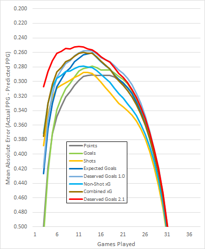
Here are the results for the average errors (MAE) between predicted and actual future points per game (PPG) for each metric.

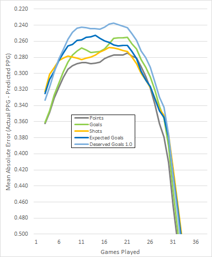
So, Deserved Goals 1.0 was pretty good. It picked up a signal quickly, and outperformed the other metrics (including Expected Goals) for the majority of the season.

Since I wrote my original blog post, a number of things have changed. Firstly, data for Expected Goals (xG) is now freely available from a number of sources. I have used FiveThirtyEight’s data for the above chart. This data was not available a few years ago.

Secondly, a second form of xG has been developed, called non-shot xG. Rather than using shots, it gives an xG value to each period of possession, meaning you get more meaningful data points quicker than using shot-based xG. Theoretically, this should give better predictions earlier in the season.

Indeed, this is what we see when we plot the non-shot xG on the chart.

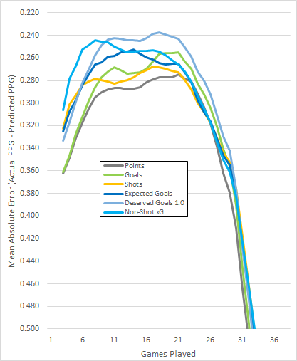
Non-Shot xG is a much better predictor than any other metric early in the season, although it is still not as good as Deserved Goals 1.0 in the latter 2 thirds of the season.

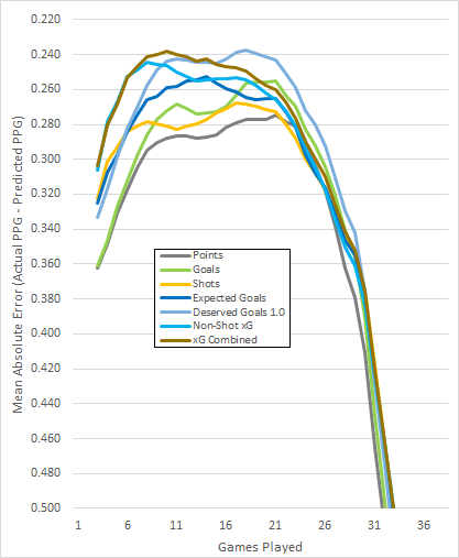
Combining the 2 versions of xG is even more powerful. Simply taking an average of the Shot-based and Non-Shot xG figures improves performance, as seen below. This will be referred to as Combined xG.

OK, so now we’ve set the challenge to beat. I want Deserved Goals 2.0 to be as powerful in the early season as Combined xG, and I want to keep the strong performance in the second half of the season.

Here’s my thought process. The original formula was as follows:

Deserved Goals 1.0 = ( Average Shots + A% of the variance ) x ( Average Conversion + B% of the variance )

I still want to use shots as the starting point, and so the initial part of the formula remains unchanged. This gives us an estimate of how good a team is at creating shooting opportunities.

( Average Shots + A% of the variance )

I want to improve early season performance by using Combined xG, so next up is an adjustment to account for how good these shots are predicted to be. For this let’s use Combined xG divided by the number of shots, for which the average will be the same as the average conversion, 11.09%. As with all parts of the formula, we will only keep a percentage of the variance from the average. This gives us an estimate of how good a team is at ensuring their shots are taken from good locations:

( Average Combined xG per shot + B% of the variance )

We then have the old conversion rate, but rather than using shots we are using Shot-based xG, so this becomes the conversion of Expected Goals into goals, which on average should be 100%. This gives us an estimate of how good a team is at converting shots into goals, controlled for the quality of the chance. You might call this finishing skill:

( Average Goals per Shot-based xG + C% of the variance )

 

The formula is therefore:

Deserved Goals 2.0 = (( Average Shots + A% of the variance ) x ( Average Combined xG per Shot + B% of the variance )) x ( Average Goals per Shot based xG + C% of the variance )

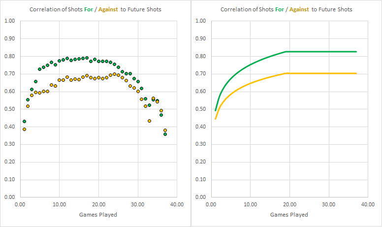
I need to select values for A, B and C. These should be a good approximation of the extent to which the 3 components are skill rather than luck. In other words, how much of the variance from the average is signal rather than noise. We would expect the ability to create shots to be mostly signal, whereas finishing skill is notoriously “noisy”, so we would expect a low %.

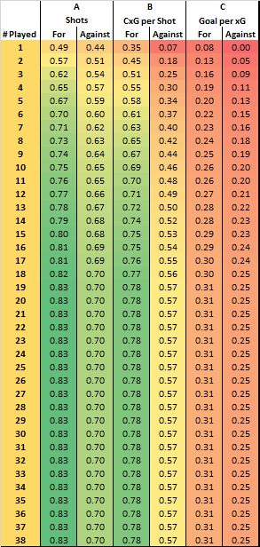
To get a rough idea of what these should be, I have calculated how much these 3 components revert to the mean between seasons, using Pearson’s R (The CORREL function in Excel).

Here are the results:

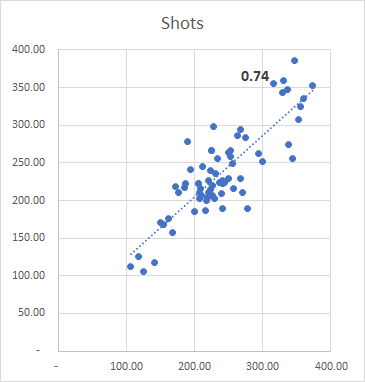
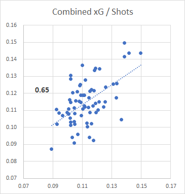
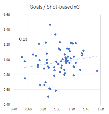
So, just using these figures would mean A=74%, B=65% and C=13%. That’s a good starting point, however looking at season-to-season correlations is a bit misleading. Teams often change personnel between seasons, so I would expect the correlations to be higher than this within a season where personnel stays mostly the same.

Let’s increase each figure a bit, to A=90%, B=75%, and C=25%, and see how the metric performs.

The final formula is therefore:

Deserved Goals 2.0 = (( Average Shots+ 90% of the variance ) x ( Average Combined xG per Shot + 75% of the variance )) x ( Average Goals per Shot-Based xG + 25% of the variance )

or:

Deserved Goals = ((453 + 90% x (Shots – 453)) x (11.09% + 75% x (Combined xG per Shot – 11.09%))) x ( 100% + 25% x (Average Goals per Shot-Based xG – 100%))

OK, so let’s see how this metric gets on.

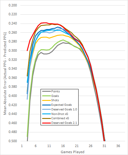
Previously the best 2 metrics were Combined xG and Deserved Goals 1.0. Here’s how Deserved Goals 2.0 compares to those:

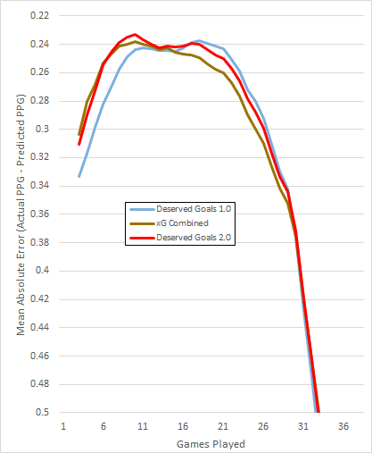
I’m classing that as a success. Deserved Goals 2.0 is much better than the original version in the early part of the season, and is on a par with Combined xG. In the latter stages it outperforms Combines xG, and is almost as good as the original version. Overall, it is the best metric of all the ones I have tested so far.

I could probably tweak the values of A, B and C to improve the results, but I think there would be a risk of over-fitting to the data.

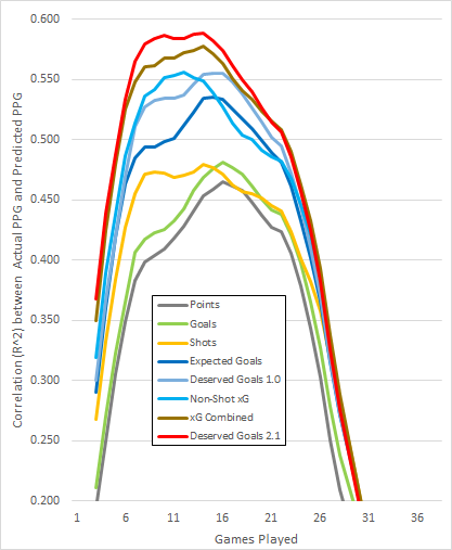
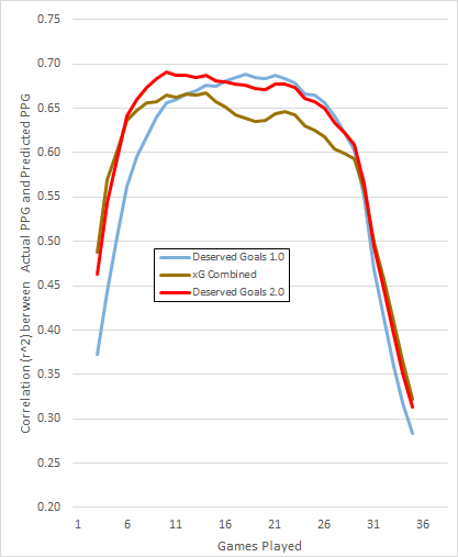
Another way of measuring the performance of predictive metrics is to use r^2 instead of average errors. This produces similar results:

If you enjoyed this post, please see part 2 here, where I develop this further.

If you have any questions, comments or suggestions, please let me know. I am on Twitter @8Yards8Feet

Data from: http://www.football-data.co.uk/ and https://projects.fivethirtyeight.com/soccer-predictions/